Comparison Front loading washing machine Vs Top loading washing machine

Front Loader (Main Advantages)
1. Wash quality - you can get a better wash quality than any top loaders (however, not as good as God-made washing machines - our hands).
2. Water/Detergent consumption - you can do a cycle of washing with comparatively less water and detergent compared to top loaders. Though you have invested a lot of money on a front loader, you can afford to save some on water and detergents.
3. Longevity - front loaders are expected to last longer than top loaders (up to 15 to 20 years of use). Ideal for consumers who believe "old is gold" and are not interested in exchange offers and/or keeping themselves updated with latest technology.

Front Loader (Main Disadvantages)
1. Price - front loaders are far expensive than top loaders. The lower-end version/model in a front loader is much more expensive than the higher-end version/model in a top loader.
2. Complex mechanism - front loaders run without a problem as long as they run, but once they land in some problem, it is forever. Never you can expect the same performance after repair that you found when you bought it. Also, bending down to load a front loader washing machine is considered inconvenient.
3. Repair cost/service - the cost involved in repairing front loaders or getting on-time repair service is a real challenge. You might have to wait as long as 20 days to 3 months to get a fault repaired and then shed a good amount of money for that repair.

Top Loader (Main Advantages)
1. User friendly - top loaders boast the comfort and convenience of any common user (non-technical housewives) who can operate the machine without any complications . Another most noted advantage across the world, especially in America and Australia, is the convenience to stand and load the machine without having to bend down as in front loaders.
2. Power consumption - power consumed by a top loader is comparatively less than a front loader, basically because of the time consumed in washing. A cycle of wash lasts for 30 to 45 minutes in a top loader while the same cycle of wash in a front loader can run up to 1 to 2 hours.
3. Maintenance - top loaders have quite simple mechanism compared to front loaders and involve more electronics than mechanical. So, any repair here might not be as expensive as repairs in front loaders and the service is also quick and affordable.

Top Loader (Main Disadvantages)
1. Wash quality - sources claim that top loaders’ wash quality is not as good as in front loaders. Since the drum in top loaders is vertical, chances are that clothes at the bottom of the drum and at the top of the drum fail to interchange positions to attain the same wash quality. (SOME BRANDS HAVE TACKLED THIS PROBLEM NOW - see below).
2. Water/Detergent consumption - top loaders consume more water and detergent compared to front loaders during a wash cycle. This is mainly because the volume of water required in a top loader to wash a certain load is much more compared to a front loader to wash the same load, thereby utilizing more detergent also.
3. Noise/Vibration - some top loaders might create vibration and some low-level noise during operation. This is mainly because the body of a top loader is lighter than a front loader and occupies lesser ground space than a front loader.

Now, having differntiated between front loaders and top loaders, I hope the above information has helped us to decide between a front loader and a top loader.

For all those who have decided to go ahead with a front loader, there is no choice in brand. In India, the obvious front loader market leader is IFB. If at all you have decided to buy a front loader, you can wisely go ahead with an IFB. However, please note that it is advisable to go for higher-end versions/models than lower-end versions/models since you might not get most of the features in lower-end versions despite paying such a huge amount.

For all those who have decided to go ahead with a top loader, there are two leading successful brands - LG and Whirlpool. Also, these two guys have worked out their latest washing machines to match with the wash quality of front loaders. LG has come up with TURBO DRUM technology, in which the drum rotates anticlockwise to the water ensuring a thorough wash cycle. Similarly, Whirlpool has come up with 1-2, 1-2 technology, in which there is an agitator in the center of the drum, which holds clothes like in hands and rubs hard to remove hardcore stains and dirt. (Please note there are some complaints that the agitator in Whirlpool twists and wrinkles the clothes leading to some wear and tear gradually).

Front loader (IFB)/Samsung//Lg or Top loader (LG/Whirlpool/Samsung) - .

The choice is yours

RAID 0, RAID 1, RAID 2, RAID 3, RAID 5, RAID6, RAID 10 Explained

RAID 0, RAID 1, RAID 5, RAID 10 Explained with Diagrams

RAID stands for Redundant Array of Inexpensive (Independent) Disks.
On most situations you will be using one of the following four levels of RAIDs.

• RAID 0
• RAID 1
• RAID 2
• RAID 3

• RAID 5
• RAID 10 (also known as RAID 1+0)

This article explains the main difference between these raid levels along with an easy to understand diagram.

In all the diagrams mentioned below:

• A, B, C, D, E and F – represents blocks
• p1, p2, and p3 – represents parity

RAID LEVEL 0

Following are the key points to remember for RAID level 0.

• Minimum 2 disks.
• Excellent performance ( as blocks are striped ).
• No redundancy ( no mirror, no parity ).
• Don’t use this for any critical system.

RAID LEVEL 1

          Following are the key points to remember for RAID level 1.

• Minimum 2 disks.
• Good performance ( no striping. no parity ).
• Excellent redundancy ( as blocks are mirrored ).

• RAID ARRAY 2

  
  
• This uses bit level striping. i.e Instead of striping the blocks across the disks, it stripes the bits across the disks.
• In the above diagram b1, b2, b3 are bits. E1, E2, E3 are error correction codes.
• You need two groups of disks. One group of disks are used to write the data, another group is used to write the error correction codes.
• This uses Hamming error correction code (ECC), and stores this information in the redundancy disks.
• When data is written to the disks, it calculates the ECC code for the data on the fly, and stripes the data bits to the data-disks, and writes the ECC code to the redundancy disks.
• When data is read from the disks, it also reads the corresponding ECC code from the redundancy disks, and checks whether the data is consistent. If required, it makes appropriate corrections on the fly.
• This uses lot of disks and can be configured in different disk configuration. Some valid configurations are 1) 10 disks for data and 4 disks for ECC 2) 4 disks for data and 3 disks for ECC
• This is not used anymore. This is expensive and implementing it in a RAID controller is complex, and ECC is redundant now-a-days, as the hard disk themselves can do this.

RAID 3

• This uses byte level striping. i.e Instead of striping the blocks across the disks, it stripes the bits across the disks.
• In the above diagram B1, B2, B3 are bytes. p1, p2, p3 are parities.
• Uses multiple data disks, and a dedicated disk to store parity.
• The disks have to spin in sync to get to the data.
• Sequential read and write will have good performance.
• Random read and write will have worst performance.
• This is not commonly used.

•  

RAID LEVEL 5

Following are the key points to remember for RAID level 5.

• Minimum 3 disks.
• Good performance ( as blocks are striped ).
• Good redundancy ( distributed parity ).
• Best cost effective option providing both performance and redundancy. Use this for DB that is heavily read oriented. Write operations will be slow.

  RAID ARRAY 6

  
  
• Just like RAID 5, this does block level striping. However, it uses dual parity.
• In the above diagram A, B, C are blocks. p1, p2, p3 are parities.
• This creates two parity blocks for each data block.
• Can handle two disk failure
• This RAID configuration is complex to implement in a RAID controller, as it has to calculate two parity data for each data block.

RAID LEVEL 10

  Following are the key points to remember for RAID level 10.

• Minimum 4 disks.
• This is also called as “stripe of mirrors”
• Excellent redundancy ( as blocks are mirrored )
• Excellent performance ( as blocks are striped )
• If you can afford the dollar, this is the BEST option for any mission critical applications (especially databases).

RAID Configuration

RAID 0

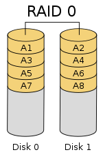
Diagram of a RAID 0 setup

A RAID 0 (also known as a stripe set or striped volume) splits data evenly across two or more disks (striped) without parity information for speed. RAID 0 was not one of the original RAID levels and provides no data redundancy. RAID 0 is normally used to increase performance, although it can also be used as a way to create a large logical disk out of two or more physical ones.
A RAID 0 can be created with disks of differing sizes, but the storage space added to the array by each disk is limited to the size of the smallest disk. For example, if a 100 GB disk is striped together with a 350 GB disk, the size of the array will be 200 GB (100 GB × 2).

The diagram shows how the data is distributed into Ax stripes to the disks. Accessing the stripes in the order A1, A2, A3, ... provides the illusion of a larger and faster drive. Once the stripe size is defined on creation it needs to be maintained at all times.

Performance

RAID 0 is also used in some computer gaming systems where performance is desired and data integrity is not very important. However, real-world tests with computer games have shown that RAID-0 performance gains are minimal, although some desktop applications will benefit.^[2][3] Another article examined these claims and concludes: "Striping does not always increase performance (in certain situations it will actually be slower than a non-RAID setup), but in most situations it will yield a significant improvement in performance." ^[4]

RAID 1

Diagram of a RAID 1 setup

An exact copy (or mirror) of a set of data on two disks. This is useful when read performance or reliability is more important than data storage capacity. Such an array can only be as big as the smallest member disk. A classic RAID 1 mirrored pair contains two disks (see reliability geometrically) over a single disk. Since each member contains a complete copy and can be addressed independently, ordinary wear-and-tear reliability is raised by the power of the number of self-contained copies.

Performance

Since all the data exists in two or more copies, each with its own hardware, the read performance can go up roughly as a linear multiple of the number of copies. That is, a RAID 1 array of two drives can be reading in two different places at the same time, though most implementations of RAID 1 do not do this.^{[5][citation needed]} To maximize performance benefits of RAID 1, independent disk controllers are recommended, one for each disk. Some refer to this practice as splitting or duplexing (for two disk arrays) or multiplexing (for arrays with more than two disks). When reading, both disks can be accessed independently and requested sectors can be split evenly between the disks. For the usual mirror of two disks, this would, in theory, double the transfer rate when reading. The apparent access time of the array would be half that of a single drive. Unlike RAID 0, this would be for all access patterns, as all the data are present on all the disks. In reality, the need to move the drive heads to the next block (to skip blocks already read by the other drives) can effectively mitigate speed advantages for sequential access. Read performance can be further improved by adding drives to the mirror. Many older IDE RAID 1 controllers read only from one disk in the pair, so their read performance is always that of a single disk. Some older RAID 1 implementations read both disks simultaneously to compare the data and detect errors. The error detection and correction on modern disks makes this less useful in environments requiring normal availability. When writing, the array performs like a single disk, as all mirrors must be written with the data. Note that these are best case performance scenarios with optimal access patterns.

RAID 2

RAID Level 2

A RAID 2 stripes data at the bit (rather than block) level, and uses a Hamming code for error correction. The disks are synchronized by the controller to spin at the same angular orientation (they reach Index at the same time), so it generally cannot service multiple requests simultaneously. Extremely high data transfer rates are possible. This is the only original level of RAID that is not currently used.^[6][7]
All hard disks eventually implemented Hamming code error correction. This made RAID 2 error correction redundant and unnecessarily complex. This level quickly became useless and is now obsolete. There are no commercial applications of RAID 2.^[6][7]

RAID 3

Diagram of a RAID 3 setup of 6-byte blocks and two parity bytes, shown are two blocks of data in different colors.

A RAID 3 uses byte-level striping with a dedicated parity disk. RAID 3 is very rare in practice. One of the characteristics of RAID 3 is that it generally cannot service multiple requests simultaneously. This happens because any single block of data will, by definition, be spread across all members of the set and will reside in the same location. So, any I/O operation requires activity on every disk and usually requires synchronized spindles.
This makes it suitable for applications that demand the highest transfer rates in long sequential reads and writes, for example uncompressed video editing. Applications that make small reads and writes from random disk locations will get the worst performance out of this level.^[7]
The requirement that all disks spin synchronously, a.k.a. lockstep, added design considerations to a level that didn't give significant advantages over other RAID levels, so it quickly became useless and is now obsolete.^[6] Both RAID 3 and RAID 4 were quickly replaced by RAID 5.^[8] RAID 3 was usually implemented in hardware, and the performance issues were addressed by using large disk caches.^[7]

RAID 4

Diagram of a RAID 4 setup with dedicated parity disk with each color representing the group of blocks in the respective parity block (a stripe)

A RAID 4 uses block-level striping with a dedicated parity disk.
In the example on the right, a read request for block A1 would be serviced by disk 0. A simultaneous read request for block B1 would have to wait, but a read request for B2 could be serviced concurrently by disk 1.
RAID 4 is very uncommon, but one enterprise level company that has previously used it is NetApp. The aforementioned performance problems were solved with their proprietary Write Anywhere File Layout (WAFL), an approach to writing data to disk locations that minimizes the conventional parity RAID write penalty. By storing system metadata (inodes, block maps, and inode maps) in the same way application data is stored, WAFL is able to write file system metadata blocks anywhere on the disk. This approach in turn allows multiple writes to be "gathered" and scheduled to the same RAID stripe—eliminating the traditional read-modify-write penalty prevalent in parity-based RAID schemes.^[9]

RAID 5

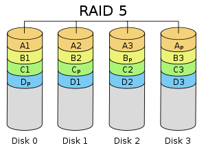
Diagram of a RAID 5 setup with distributed parity with each color representing the group of blocks in the respective parity block (a stripe). This diagram shows left asymmetric algorithm

A RAID 5 comprises block-level striping with distributed parity. Unlike in RAID 4, parity information is distributed among the drives. It requires that all drives but one be present to operate. Upon failure of a single drive, subsequent reads can be calculated from the distributed parity such that no data is lost. RAID 5 requires at least three disks.^[10]

RAID 6

Diagram of a RAID 6 setup, which is identical to RAID 5 other than the addition of a second parity block

RAID 6 extends RAID 5 by adding an additional parity block; thus it uses block-level striping with two parity blocks distributed across all member disks.

Performance (speed)

RAID 6 does not have a performance penalty for read operations, but it does have a performance penalty on write operations because of the overhead associated with parity calculations. Performance varies greatly depending on how RAID 6 is implemented in the manufacturer's storage architecture – in software, firmware or by using firmware and specialized ASICs for intensive parity calculations. It can be as fast as a RAID-5 system with one fewer drive (same number of data drives).^[11]

Implementation

According to the Storage Networking Industry Association (SNIA), the definition of RAID 6 is: "Any form of RAID that can continue to execute read and write requests to all of a RAID array's virtual disks in the presence of any two concurrent disk failures. Several methods, including dual check data computations (parity and Reed-Solomon), orthogonal dual parity check data and diagonal parity, have been used to implement RAID Level 6."^[12]

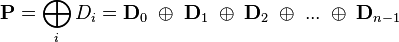
Computing parity

Two different syndromes need to be computed in order to allow the loss of any two drives. One of them, P can be the simple XOR of the data across the stripes, as with RAID 5. A second, independent syndrome is more complicated and requires the assistance of field theory.
To deal with this, the Galois field is introduced with , where for a suitable irreducible polynomial of degree . A chunk of data can be written as in base 2 where each is either 0 or 1. This is chosen to correspond with the element in the Galois field. Let correspond to the stripes of data across hard drives encoded as field elements in this manner (in practice they would probably be broken into byte-sized chunks). If is some generator of the field and denotes addition in the field while concatenation denotes multiplication, then and may be computed as follows ( denotes the number of data disks):

For a computer scientist, a good way to think about this is that is a bitwise XOR operator and is the action of a linear feedback shift register on a chunk of data. Thus, in the formula above,^[13] the calculation of P is just the XOR of each stripe. This is because addition in any characteristic two finite field reduces to the XOR operation. The computation of Q is the XOR of a shifted version of each stripe.
Mathematically, the generator is an element of the field such that is different for each nonnegative satisfying .
If one data drive is lost, the data can be recomputed from P just like with RAID 5. If two data drives are lost or a data drive and the drive containing P are lost, the data can be recovered from P and Q or from just Q, respectively, using a more complex process. Working out the details is extremely hard with field theory. Suppose that and are the lost values with . Using the other values of , constants and may be found so that and :

Multiplying both sides of the equation for by and adding to the former equation yields and thus a solution for , which may be used to compute .
The computation of Q is CPU intensive compared to the simplicity of P. Thus, a RAID 6 implemented in software will have a more significant effect on system performance, and a hardware solution will be more complex.